Hands on approach to Quantum Information Processing 101, using declarative syntax.

I’ve always been a pretty vocal proponent of getting one’s hands dirty prior to studying theory. It makes much more sense to be exposed to abstract ideas, when you can understand their applications and value.

This holds true for both Computer Science and Quantum Physics. During my time at FSU and UIUC, I experienced many CS students who had no idea how to apply in real life the knowledge they gained at a hefty premium.

With that said, this little exercise will serve as both an introduction to quantum gates as well as “I wish they told me” of what I personally found to be missing from many Quantum Physics books.

It is no my goal to reinvent the wheel and compete with excellent libraries like qiskit. I have – however – experienced the attrition rate of IBM’s summer quantum school, which I partially attribute to a steep curve they throw at potential candidates.

Goal for Part 1

I want to implement a very simple circuit simulator and QASM parser. To begin with, we’re going to work with 1 qbit at a time. This simply means that all components will be daisy chained and sandwiched between an input signal (0 or 1) and output measurement.

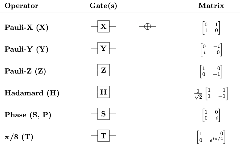
These are the gates I am going to implement in Part 1. They all have only 1 input:

For implementation, I will use Haskell. I want to force my hand into a declarative syntax and later on compare it with iterative approach.

References

Those usually come at the end – but since it’s a 101 approach, there are two sources I need to mention:

• http://learnyouahaskell.com/ – The best intro to functional programming. In Part 1, I will use concepts up to Chapter 8 (ADTs)
• https://qiskit.org/learn/course/introduction-course – Qiskit intro course, for the foundations of Quantum Physics

Quantum Information and State

In order to process information, we need to somehow represent it in our code. With classical digital data, it’s pretty straight forward, as we’re simply using the values of 0 and 1 as building blocks. Those can be easily encoded using voltage, frequency, light, card holes and Minecraft blocks.

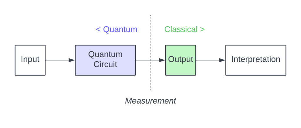
So how is Quantum world different? At the end of the day, we still need to be able to extract the output from our processing machine. And for us to understand that data (whether in a single reading or a series of experiments), it needs to be measured and interpreted.

That output therefore has to be classical. The quantum phenomena is what happens inside our circuits during information processing. Once our algorithm concludes, we perform a measurement, which collapses the quantum fabric into an everyday boring 0 or 1.

The main difference between classical and quantum circuits is their determinism. While the former are fully deterministic (meaning if we send “0” to a circuit of classical gates, we will always get the same output), quantum contraptions will yield outputs (0 or 1) with some probabilities.

For instance: a qbit |0> sent through a Hadamard gate will come out either as 0 (50% chance) or 1 (50% chance). This is real non-determinism, as opposed to various pseudo-random generators we rely on for our everyday cryptography.

This non-deterministic nature of our circuit is removed when we perform a reading (a.k.a. wave function collapse). After all, we cannot observe two different outputs at the same time. Like the infamous cat, it must be either dead or alive once we open the box. Therefore, to confirm if the outcome probabilities match our expected distribution, we have to perform a series of tests.

Beyond Probabilities

To merely account for a chance of a given output of our circuit component would not be enough to fully describe and simulate the quantum phenomena. If that was the case, we could simply multiply the probabilities of daisy-chained elements and get the final distribution of 0 and 1.

If we were to only ever simulate one gate at a time, this would be sufficient. But the moment we connect them to one another and have our quantum states interact, we’d be in trouble. Some of the observed distributions would not match our expected values. For instance: 2 Hadamard gates one after another would not result in a 50/50 distribution of 0 and 1.

For a complete picture, we need to expand the quantitative description of our gate outputs (and therefore, the circuit state in general) into a two-dimensional value. This extra layer of information does not correspond to a directly observable feature. It was simply discovered through experiments and observations of quantum interactions, just like most things in physics.

So an easy way to think about circuit evolution is: treat classical ones as 1-D and quantum as 2-D. This does not answer the question why they behave in a certain way, but it does allow us to predict their behavior (outcome probability distribution).

This is not in any way different from Newtonian physics. All the formulas we study in high school are merely and attempt to mathematically model the world we live in. They don’t address the metaphysical question of “why”. Math is also a very useful band-aid to fill in the gaps of unknown, like we do with dark matter and energy.

Going back to our circuit state: there are two isomorphic ways to describe two-dimensional values.

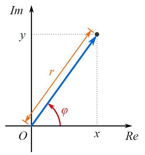
To locate the dot on our 2-D plane, we can use either:

• the imaginary number notation, in this case x + bi, where i² = -1
• phase φ and magnitude r, where φ is the angle with positive real axis.

In Part 1, we are going to use phases and magnitudes. We will implement basic circuit with φ as a whole degree (0-359) to show the underlying logic. This will certainly introduce some rounding errors, which will be addressed in future parts as we switch to imaginary numbers.

Basic Types

We are now ready to define some very basic building blocks of our circuits.

type QBit = Integer
type Phase = Integer
type Value = Float

Nothing too crazy here. Value is our probability magnitude. We square it to get the actual probability.

We can now define a complete 1-qbit state of our circuit:

type PhaseValues = Map Phase Value
type QBitPhases = (QBit, PhaseValues)
type BinaryState = [QBitPhases]

PhaseValues is simply a bunch of vectors anchored at (0, 0). For BinaryState to represent an actual circuit state, it would contain either one (single qbit with a certainty of 100%) or two QbitPhases whose probabilities add up to 100%.

The post-measurement output can be described as:

type StateProbs = [(QBit, Float)]

Again, we expect those to add up to 100%.

Finally, we can define our circuit elements and the circuit itself:

data CirElem = GateH CirElem
    | GateX CirElem
    | GateY CirElem
    | GateZ CirElem
    | GateS CirElem
    | GateT CirElem
    | CInput QBit
    | COutput CirElem deriving (Show, Eq)

type Circuit = [CirElem]

The Gate ADT uses typical linked list constructors to interconnect the elements with one another, for instance we can define a simple circuit as:

COutput (GateH (GateH (GateH (GateH (CInput 0)))))

The problem with this notation is that it needs to be read backwards (from inside out). We can address it by introducing a new infix operator -:

(-:) :: a -> (a -> b) -> b
x -: f = f x

It’s very straightforward: it takes an argument of type “a” and a function which operates on that argument and returns the output of the function applied to it. With it, we can rewrite our circuit as:

(CInput 0) -: GateH -: GateH -: GateH -: GateH -: COutput

Helper Functions

Our goal is to simulate the behavior of those six gates which operate on 1 qbit. Mathematically, a gate is simply a numerical operation on a given state vector. It can be described using linear algebra and matrix operations, which we will do in a later part. Alternatively, we can think of gates as taking an input state vector and emitting a new output based on its magnitude and phase. This will be done separately for qbits |0> and |1> vectors of the input state.

To implement this, we need some vary basic geometric functions that operate on vectors. Let’s start with a phase shifter:

shiftPhases :: PhaseValues -> Phase -> PhaseValues
shiftPhases pvs s = Map.fromList [(mod (phase + s) 360, value) | (phase, value) <- Map.toList $ pvs]

It is fairly straightforward. We use list comprehension, so we need to convert from map to list and then back to map. Also, we mod the result over 360, since that is the total number of degrees in a full circle.

Then, we need radians <> degrees converters:

degToRad :: Phase -> Float
degToRad d = df * (pi / 180)
    where df = fromIntegral d :: Float

radToDeg :: Float -> Phase
radToDeg r = round $ r * (180 / pi)

When we add a new vector to an existing map, it might turn out there already is a vector at this degree (remember, we’re using whole degrees here). In that case, we might simply increase its magnitude:

addPhaseValue :: Phase -> Value -> PhaseValues -> PhaseValues
addPhaseValue ph val pv =
    case Map.lookup ph pv of
        Just x -> Map.adjust (+ x) ph pv
        _ -> Map.insert ph val pv

Finally, we need to be able to add two vectors together, which we’ll need to calculate the final probability of a state:

mergeVectors :: (Phase, Value) -> (Phase, Value) -> (Phase, Value)
mergeVectors (0, 0) b = b
mergeVectors a (0, 0) = a
mergeVectors (ap, av) (bp, bv) =
    let sx = (av * cos (degToRad ap)) + (bv * cos (degToRad bp))
        sy = (av * sin (degToRad ap)) + (bv * sin (degToRad bp))
        adjDeg = (case (sx < 0) of True -> 180
                                   False -> 0)
    in (mod ((radToDeg (atan (sy / sx))) + (adjDeg)) 360, sqrt (sx ** 2 + sy ** 2))